How we set realistic targets for research tasks
Agents are moving into research
The field is turning agents toward research itself. It started with AI research: MLE-bench grades agents on Kaggle competitions [1], RE-Bench pits them against human experts on open AI research problems [2], and PaperBench asks them to rebuild published papers from scratch [3]. The same push has reached the life sciences, with BioMysteryBench [4] and OpenAI’s LifeSciBench [5] and GeneBench-Pro [6], and materials science, with CompMat-Bench [7].
Scores on these benchmarks are often low, and it is tempting to read this as evidence that models are not ready yet. But research tasks have an awkward property: often, nobody knows the right answer. Nobody has the best possible ranking of 5,000 drug candidates. Even the best lab in the world has only the best method available today, and next year someone may have a better one. A low score, then, may say as much about the task as about the model. The key question is whether the information available to the agent is enough to support a high score. In our second case study, the answer key uses a part of each antibody that the agent never sees, making some errors unavoidable.
Why the score range matters
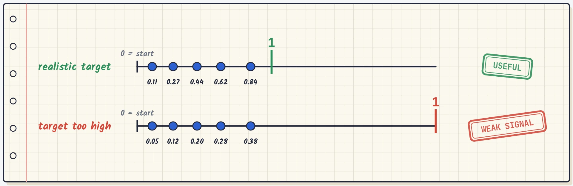
One way to evaluate open-ended research tasks is to measure progress between a starting solution and a strong reference solution. RE-Bench does this by assigning a score of 0 to the starting solution and 1 to a strong reference solution [2]. We use the same approach. Reward 0 corresponds to a naive baseline that the agent is asked to improve on. It is deliberately simple, so most standard frontier agents should be able to outperform it. Reward 1 corresponds to the best score we estimate a strong solver could achieve.
The starting score is straightforward to measure: we run the baseline and record its result. The target is harder. It represents a solution that may not exist yet, so we have to estimate how well a strong solver could do. An inaccurate estimate can distort the rewards and, in turn, how we interpret agent performance.
The reward is calculated using three quantities:
- score: The agent’s score on the hidden test set.
- start: The score of the naive baseline given to the agent. It is deliberately simple and should be beatable by most standard frontier agents. It defines reward 0.
- target: Our estimate of the best score a strong solver could realistically achieve. It defines reward 1.
reward = (score − start) / (target − start)In other words, the reward measures how much of the gap between the starting point and the target the agent closes. If the target is overestimated, the gap becomes wider, and the same agent performance receives a lower reward. This matters in three ways:
- The target sets the scale of every reward. An overestimated target shrinks every reward by the same factor. In case study 1, rewards were about four times smaller than they should have been (k = 0.24). Good runs look like failures, and the gaps between agents shrink by the same factor.
- An unrealistic target leaves little or no headroom for learning. When a target is not achievable under the given environment constraints, agents may make meaningful progress but still remain far from the target. In the extreme case, where no attempt can reach the target and rewards are pass/fail, every attempt receives a score of 0. GRPO then assigns zero advantage to every attempt, leaving no useful learning signal.
- A wrong target can distort the balance between rewards. When rewards are combined using fixed weights, an overestimated target shrinks only the task reward, giving other rewards a larger share of the learning signal. For example, in training recipes such as DeepSeek-R1, the format reward is added to the accuracy reward [8]. Normalizing each reward separately before combining them can help avoid this problem [9].
An optimistic target first, then an audit
We want every research task to have a target: an estimate of the best score a strong solver could achieve. Since there is no known answer to look up, we start by building an optimistic oracle. It is the best score we can obtain using information the agent never receives, such as hidden answers, withheld columns, or additional experiments. This gives us an upper bound, but the environment the agent operates in is not perfect, so some of that score may be out of reach. For example, in our second case study, the answer key relies on the antibody’s light chain, but the agent sees only the heavy chain. This information gap is a limitation of the environment, which makes some errors unavoidable.
We audit this estimate using a validation notebook, a Jupyter notebook that accompanies every task. The notebook performs exploratory data analysis and targeted experiments on the underlying data to investigate whether the proposed target is supported by the resources available to the agent. It looks for meaningful signals and exploitable structure, and runs checks for unsupported assumptions, or information that would not be available to the agent. These checks help establish whether the proposed score is genuinely reachable using the agent’s inputs. The notebook must ultimately either support the proposed target or contradict it. If it contradicts the target, it must identify the highest score supported by the available evidence.
This approach follows BioMysteryBench, which also required task authors to demonstrate that the signal actually exists in the data:
“To minimize inherently unsolvable questions while still leaving room for those that might be AI-solvable, we required each question author to submit a validation notebook demonstrating that the signal does, in fact, exist in the data (even if finding it from scratch might be difficult). Think of this as the high-school algebra principle: verifying an answer is much easier than deriving one.”
For a task without an oracle, this notebook is the most important audit point. If the target is wrong, every reward on the task is wrong with it.
We use three layers of review, with each layer checking the work of the previous one:
- An agent writes the notebook. Starting from the optimistic target, it explores the real data, runs experiments, and tries to find evidence that challenges the estimate.
- A separate QA agent audits the notebook. It checks the analysis, validation logic, data leakage, and assumptions.
- A PhD-level domain expert reviews both. They assess whether the scientific reasoning holds up and whether the proposed solution and its score are justified.
The three case studies below come from chemistry, biology and AI research. The first is hit triage in drug discovery: deciding which results from a chemical screen are worth following up. The second is antibody discovery: grouping a patient’s immune cells into families to find antibodies worth developing. The third is kernel optimization: making a GPU program for language-model inference run faster.
Case study 1: hit triage in a drug screen
Task
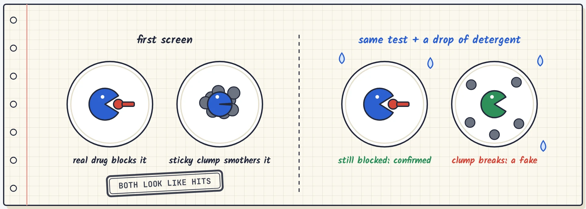
A lab tests thousands of chemicals against an enzyme from the parasite that causes Chagas disease. Chemicals that slow the enzyme down are called hits. But many hits are false positives. Some compounds form sticky clumps that interfere with the enzyme and make it appear inhibited. Following up on these false positives wastes time and money.
Think of it as spam filtering for chemistry. The agent gets 5,323 hits and must rank them, with the most likely real hits at the top. Only about 7% are real. The answer key comes from a second experiment the agent never sees: the same test repeated with a drop of detergent. Detergent breaks up the clumps, so false positives stop working while genuine inhibitors continue to work.
For each hit, the agent sees its dose-response curve (how strongly and how steeply it acts), about a dozen computed properties such as size and greasiness, and its chemical structure. It also gets about 10,000 practice hits, of which 3,670 have known answers. We score the agent using average precision, which rewards putting real hits near the top of the ranking. A random ranking scores about 0.07, the fraction of hits that are real. A perfect ranking scores 1.0.
Starting solution
The starting solution was produced by a deliberately naive agent, serving as the baseline that the evaluated agent is expected to improve on. It trains decision tree models on the practice answers, using dose-response curve shapes, computed properties, simple features of the chemical structures, and the density of each compound’s chemical neighbourhood. It scores 0.3792 on the hidden hits.
Optimistic target and validation approach
To establish an optimistic target, we first give an agent privileged access to the hidden answers and ask it to build the best solution it can. The agent splits the hidden hits into five parts, trains on four, and predicts the fifth, repeating this for each part. However, many hidden compounds have near-copies elsewhere in the hidden set, so this setup introduces test leakage: the model can learn from the answers of near-identical compounds before predicting them. This gives a score of 0.7404, an optimistic estimate that benefits from information the evaluated agent never receives.
The validation agent then examines this optimistic approach, looking for reasons why the score might not be achievable using only the information available to the evaluated agent. The three steps below show what it found.
Step 1: Leakage check (0.7404 rejected)
To test whether 0.74 was achievable, the notebook ran the same code using only the answers available to the agent. The score dropped from 0.7404 to 0.4012. That means roughly 0.34 of the score came from answers the agent never sees. The effect becomes clearer as we give the model access to more hidden answers: its score rises from 0.40 to 0.57, then 0.68, and finally 0.74.
The main source of leakage was near-duplicate compounds. 42% of hidden compounds have another compound at least 70% similar to them elsewhere in the hidden set, compared with just 1% that have such a match among the practice answers. This gives the model an easy shortcut: if it knows the answer for one compound, it can use that answer to predict the other. To measure how much this matters, the notebook tested a simple nearest-neighbour baseline that copies the answer of the most similar compound. It scored 0.13 using the practice answers, but 0.49 using the hidden answers.
Step 2: Random cross-validation (0.5278 rejected)
Next, the notebook trained a model using only the practice answers. It kept near-twins together in each split to prevent the model from learning an answer from a near-identical compound in the test set. This gave a score of 0.5278.
However, the random splits introduced another problem: compounds from the same library could appear in both the training and test sets. The model was therefore evaluated on libraries it had already seen. The hidden hits, by contrast, come from libraries that are almost entirely absent from the practice answers. This matters because hit rates vary widely across libraries. Among practice libraries with at least 10 compounds, the fraction of real hits ranges from 0% to 45%. A model could therefore score well by learning which libraries tend to contain real hits, rather than learning the chemistry that distinguishes real hits from false positives. In effect, the 0.5278 score came from a much easier test than the one the agent actually faces.
Step 3: Leave-one-library-out validation (0.4653 adopted)
To remove that last advantage, the notebook held out one entire practice library at a time, trained on the rest, and tested on the held-out library. This better matches the conditions the agent faces on the hidden set. The raw score was 0.4110.
There was one more difference to account for: 5.2% of the practice hits are real, compared with 7.0% in the hidden set. This matters because average precision depends on the fraction of real hits in a dataset. Even a random ranking scores roughly this fraction, so a higher share of real hits tends to produce a higher score. To make the two sets comparable, the notebook removed some false positives from the practice data until real hits made up 7.0% of the set. This increased the score by 0.054, from 0.4110 to 0.4653.
The final target reflects two corrections: removing the advantage of seeing familiar libraries and accounting for the difference in hit rates between the practice and hidden sets.
Case study 2: grouping immune cells for antibody discovery
Task
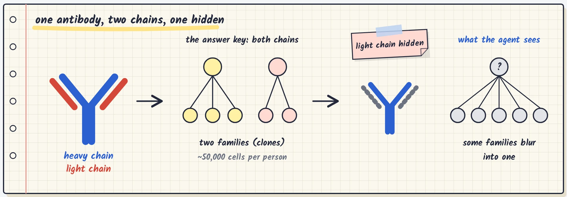
Many modern drugs are antibodies, and one way to discover promising ones is to study the immune cells of people who have fought off an infection. When an immune cell recognises an invader, it can multiply, producing a family of related cells called a clone. By grouping roughly 50,000 cells from each person into these clones, researchers can track the immune response and identify antibody families worth investigating.
Each cell carries an antibody made of two parts: a heavy chain and a light chain. The answer key groups two cells together only if both chains are sufficiently similar. The agent, however, sees only the heavy chain, which is what most real studies sequence [10]. Its task is to assign every cell to a clone using that information alone. We evaluate its predictions using pairwise F1: for every pair of cells, the score measures whether the agent correctly predicts that they belong to the same clone or to different clones. A perfect grouping scores 1.0.
Starting solution
We use the standard approach from the widely used Change-O toolkit [11] as our starting point. Although the method has access to the full heavy-chain table, it relies on just three features: the V gene, the J gene, and the junction length and sequence.
The method works in three steps:
- Initial grouping: Cells are grouped by their V gene, J gene, and junction length.
- Pairwise comparison: Within each group, two cells are linked if the proportion of mismatched letters in their junction sequences falls below a fixed threshold.
- Family assignment: These links are treated as connected components. If A is linked to B, and B is linked to C, all three cells are assigned to the same family.
Using this approach, the method achieves a score of 0.8641 on the held-out samples.
Sources of ambiguity
There are three cases that make grouping cells into families difficult:
- Identical heavy chains, different families: This is rare, but it can happen. The light chain may be the only feature that distinguishes the two families.
- Different heavy chains, same family: This is common. As cells multiply, their antibody sequences accumulate mutations, so members of the same family may have different heavy chains.
- Similar heavy chains, different families: Unrelated cells can use the same gene segments and end up with very similar sequences.
This creates a difficult distinction: two heavy chains that differ by only a few letters may belong to the same family, or they may come from entirely unrelated cells.
Step 1: Information limit of the heavy chain (1.0 rejected)
A program that uses only heavy chains cannot achieve a perfect score of 1.0. To do so, it would need to classify every pair correctly, but some cells have identical heavy chains and belong to different families because their light chains differ.
Since the program sees identical inputs for these cells, it has no way to distinguish them and must assign them the same relationship. This makes at least some classification errors unavoidable. The notebook starts with estimating the impact of these cases. Under its assumptions, a heavy-chain-only method has a maximum achievable score of approximately 0.999.
Step 2: Ceiling for the standard method (0.8922 adopted)
The 0.999 ceiling from Step 1 assumes that every uncertain pair can be resolved correctly. But the standard Change-O method uses only a limited set of features. To estimate a more realistic ceiling, the notebook considers four pieces of information for each pair of cells: whether they share an initial bucket, their junction lengths, the distance between their junction sequences, and the distance between them through a chain of links.
Change-O uses a simple rule: if two cells’ junction distance is below a fixed cut-off, they are assigned to the same family. The notebook asks how well the best possible rule using the same four features could perform. It first groups pairs with identical values for all four features. A rule that sees only these features cannot distinguish between pairs in the same group, so it must assign them all the same label. The hidden answers show how each group actually splits. For example, if a group contains 40 pairs, of which 30 belong to the same family and 10 do not, the best possible decision is to label all 40 as “same family.” This gets 30 right, while the remaining 10 errors are unavoidable. The notebook repeats this for every group, choosing whichever label is correct for the majority of pairs. This gives a maximum score of 0.8922 for any rule using these four features. The remaining errors come from groups where pairs with identical feature values have different true labels.
The two steps help us understand where the remaining errors come from. The first accounts for information that is missing when a method sees only heavy chains. The second accounts for the limitations of the four features used by Change-O. The resulting score of 0.8922 gives us a realistic upper bound.
Case study 3: speeding up an attention kernel for AI research
Task
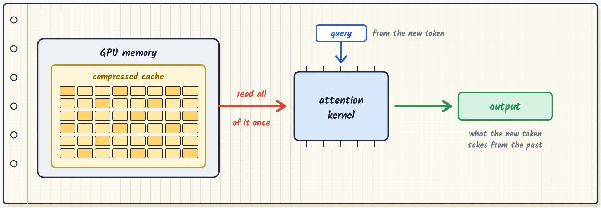
When a language model generates text, it produces one token at a time. To generate each new token, it looks back at the cache of previous tokens. Some recent models compress the cache to reduce memory usage. One example is DeepSeek’s multi-head latent attention (MLA) [12].
The agent must write a GPU kernel that performs this computation. Given the new token’s query, the compressed cache, and two matrices used to reconstruct the original representations, the kernel must produce an attention output within 2% of the reference result. The grader tests the kernel on 128 cases, varying the number of sequences processed at once (1 to 32) and the number of cached tokens (1,024 to 32,768), and scores it based on total execution time across all cases on a single NVIDIA H100 GPU. Faster kernels score better, but the achievable speedup is unknown.
Starting solution
The starting implementation uses plain PyTorch. It first unpacks the entire cache and then computes attention, taking 25 ms across all 128 test cases. The fastest result came from OpenAI’s GPT-6-Astra at 1.99 ms, followed by Opus 5.5 at 2.23 ms.
Optimistic target and validation approach
For this kernel, most of the execution time is spent reading the cache from GPU memory and the actual calculations account for only a small fraction of the time.
Across the 128 test cases, the cache contains 2.19 GB of data. The H100’s datasheet lists a memory bandwidth of 3.35 TB/s. At that speed, reading the entire cache once would take 0.654 ms. This gives us an optimistic target: a perfect kernel that reads every byte exactly once and adds no overhead.
The validation notebook tests whether this target is realistic without implementing an attention kernel. It first establishes that a correct kernel must read the entire cache, since every cache value can affect the output. The DeepSeek-V2 paper describes a technique that avoids unpacking the cache [12], but this reduces computation, not memory reads. The notebook also examines two possible shortcuts and finds that neither helps much. Even with the 2% error allowance, a kernel can skip only about 0.1% of the reads.
Step 1: Datasheet memory speed (0.654 rejected)
The memory bandwidth listed in the datasheet is a theoretical maximum. To measure what the GPU can actually achieve, the notebook ran 18 small kernels that only read memory, using the same settings as the grader. The fastest reached 3.13 TB/s, about 93% of the datasheet figure. Even allowing for both shortcuts, reaching 0.654 ms would require at least 3.27 TB/s, higher than any measured result.
Step 2: Measured memory speed (0.705 adopted)
At the measured bandwidth of 3.13 TB/s, reading all the data a correct kernel needs (2.21 GB, including the query and the two matrices) takes 0.705 ms. Unlike the datasheet-based target, this figure is supported by actual measurements, so the notebook adopts it as the new target.
There is one important complication: how the kernels are launched. The grader calls the agent’s code separately for each test case, so every case needs at least one kernel launch. Each launch costs about one microsecond, and by default, kernels run one after another. With 128 cases, even a solution using just one kernel per case would take around 1 ms. The 0.705 ms target assumes that kernels from different cases can overlap, keeping the GPU busy. The H100 supports this through programmatic dependent launch [13], and the notebook found no evidence that this approach is infeasible here. Neither of the runs we inspected uses it.
The notebook therefore keeps 0.705 ms as its target, even though the fastest observed run takes 1.99 ms. Reaching this target would require both fewer kernel launches per case and overlapping work across cases.
References
- Chan, J.S., et al. “MLE-bench: Evaluating Machine Learning Agents on Machine Learning Engineering.” arXiv:2410.07095 (2024). arxiv.org/abs/2410.07095
- Wijk, H., et al. “RE-Bench: Evaluating frontier AI R&D capabilities of language model agents against human experts.” arXiv:2411.15114 (2024). arxiv.org/abs/2411.15114
- Starace, G., et al. “PaperBench: Evaluating AI’s Ability to Replicate AI Research.” arXiv:2504.01848 (2025). arxiv.org/abs/2504.01848
- Anthropic. “Evaluating Claude’s bioinformatics research capabilities with BioMysteryBench.” April 2026. anthropic.com/research
- OpenAI. “Introducing LifeSciBench.” June 2026. openai.com/index/introducing-life-sci-bench
- OpenAI. “Introducing GeneBench-Pro.” June 2026. openai.com/index/introducing-genebench-pro
- Zhang, C., et al. “CompMat-Bench: Benchmarking AI Agents for Computational Materials Science.” arXiv:2610.00636 (2026). arxiv.org/abs/2610.00636
- DeepSeek-AI. “DeepSeek-R1: Incentivizing Reasoning Capability in LLMs via Reinforcement Learning.” arXiv:2501.12948 (2025). arxiv.org/abs/2501.12948
- Liu, S.-Y., et al. “GDPO: Group reward-Decoupled Normalization Policy Optimization for Multi-reward RL Optimization.” arXiv:2601.05242 (2026). arxiv.org/abs/2601.05242
- Zhou, J.Q., Kleinstein, S.H. “Cutting Edge: Ig H chains are sufficient to determine most B cell clonal relationships.” J. Immunol. 203:1687–1692 (2019). doi.org/10.4049/jimmunol.1900666
- Gupta, N.T., et al. “Change-O: a toolkit for analyzing large-scale B cell immunoglobulin repertoire sequencing data.” Bioinformatics 31:3356–3358 (2015). doi.org/10.1093/bioinformatics/btv359
- DeepSeek-AI. “DeepSeek-V2: A Strong, Economical, and Efficient Mixture-of-Experts Language Model.” arXiv:2405.04434 (2024). arxiv.org/abs/2405.04434
- NVIDIA. “Programmatic Dependent Launch and Synchronization.” CUDA Programming Guide. docs.nvidia.com